Sample datasets
Explore drone LiDAR datasets
6 public drone LiDAR captures, from a Los Angeles debris basin to oak woodland, a restored stream, rangeland, and farm fields in Guatemala. Switch datasets inside the viewer, color points by elevation or class, strip away vegetation where a terrain model is published, draw contours, and click the ground to read elevations.
Third-party sample data. Collected and published by research teams at Caltech, San Diego State University, Virginia Tech, and Missouri University of Science and Technology under CC BY 4.0 or CC0 licenses, and shown here so you can see what drone LiDAR deliverables look like. None of it is Twinn Digital project work. Sources and licenses
6 datasets · 2M points each · first load 15.6 MB
Data from OpenTopography, thinned and re-encoded for the web. Credits and licenses for each dataset are listed below.
In the viewer
6 datasets, different sites and sensors
Each one shows what a drone LiDAR capture produces on a different kind of ground. Layers vary with what each research team published.
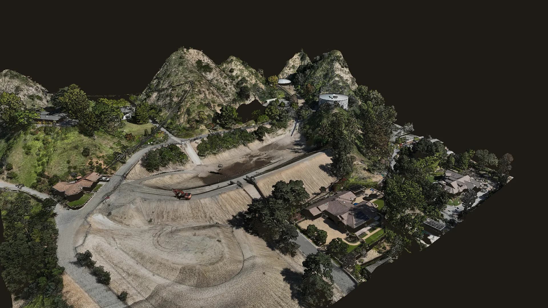
Auburn debris basin
Sierra Madre, Los Angeles County, CA
Debris basin, dam, chaparral slopes, homes.
- Captured
- Feb 2026
- Source density
- ~159 pts/m²
- Area shown
- 7.0 ha
- License
- CC BY 4.0
- Sensor
- DJI Zenmuse L2 on DJI Matrice 350 RTK
Point cloud · True color · Terrain + contours · Ortho
Volcan Mountain oak woodland
Volcan Mountain Wilderness Preserve, San Diego County, CA
Montane oak woodland and chaparral.
- Captured
- Oct 2024
- Source density
- ~1,022 pts/m²
- Area shown
- 6.0 ha
- License
- CC BY 4.0
Point cloud · True color
Stroubles Creek stream corridor
Virginia Tech StREAM Lab, Blacksburg, VA
Restored stream, riparian forest, floodplain.
- Captured
- Aug 2024
- Source density
- ~1,187 pts/m²
- Area shown
- 8.4 ha
- License
- CC BY 4.0
- Sensor
- DJI Zenmuse L1 on DJI Matrice 350 RTK
Point cloud · True color · Classified · Terrain + contours
Dawson Los Monos pasture
Dawson Los Monos Canyon Reserve, San Diego County, CA
Grazed pasture, oaks, coastal sage scrub.
- Captured
- Jul 2024
- Source density
- ~1,877 pts/m²
- Area shown
- 4.3 ha
- License
- CC0 1.0
Point cloud · True color
Dangermond Preserve rangeland
Jack and Laura Dangermond Preserve, Santa Barbara County, CA
Coastal rangeland and grazing plots.
- Captured
- Sep 2024
- Source density
- ~448 pts/m²
- Area shown
- 7.5 ha
- License
- CC0 1.0
Point cloud · True color
Motagua Valley melon farm
Near Estanzuela, Zacapa, Guatemala
Farm fields along an active fault zone.
- Captured
- Jan 2024
- Source density
- ~129 pts/m²
- Area shown
- 21.9 ha
- License
- CC BY 4.0
Point cloud · Classified · Terrain + contours
What you're looking at
The layers a LiDAR flight produces
A drone LiDAR flight produces more than a point cloud. These are the layers in the samples and the formats they are typically handed over in.
Point cloud
Every laser return as a 3D point, colored by the onboard camera where the dataset includes it. The source captures range from about 130 to 1,900 points per square meter; the viewer shows a 2-million-point sample of each (1 million on phones).
LAS / LAZ
Classification
Points labeled as ground, vegetation, buildings, or water. Ground points are what a bare-earth surface is built from. Two of the samples are classified; switch Point color to Classes to see it.
Classified LAS / LAZ
Bare-earth terrain model and contours
A ground-only surface with vegetation and most structures removed, with 1 ft, 2 ft, or 5 ft contours traced from it. It is the surface grading, drainage, and site layout are designed against.
GeoTIFF DTM, DXF / DWG, Shapefile
Orthomosaic
A georeferenced aerial image draped over the terrain for context. The Auburn sample includes one, captured at about 3.3 cm per pixel (shown here at reduced resolution).
GeoTIFF
Put the data to work
Measure it yourself
Public LiDAR like these samples powers a set of interactive 3D tools. Orbit real terrain and get volumes, movement, sections and files for CAD.
Debris basin storm tracker
Five real drone LiDAR surveys of one basin below the Eaton Fire, Oct 2025 to Feb 2026. Scrub through the storms, set your cleanout trigger, and export a status sheet.
Landfill airspace and life
Two real lidar flights of one landfill, eight years apart. Set the final grade, draw the permit footprint, and get airspace used, airspace left and years of life.
Stockpile inventory in 3D
Click a pile on a modelled sample yard with known volumes. The toe and base come from the surface; set the material and get cubic yards, tons and the change since last month.
Grading vs design in 3D
Real lidar before and after a mass-grading job. Draw pay areas on the 3D surface and get cut, fill and net, with sections and an export.
Slope movement monitor
A real, active landslide flown twice by USGS lidar. Arrows show how far the ground moved; set your alert limit and drop monitoring points anywhere.
3D LiDAR measure and export
Classified point clouds you can orbit, measure and cut sections through. Download the points or contours for the area you need.
Reading the samples
What to notice
Ground under the trees. On Stroubles Creek, color the points by Classes: the ground points continue under the riparian canopy, which is what lets a bare-earth surface be built on vegetated sites.
Gaps are information too. The dark hole in the Auburn basin is standing water. Water absorbs the laser, so LiDAR returns few or no points from it.
This is research data, not finished design deliverables. Several samples are unclassified, terrain models appear only where the research team published one, and some published models still include structures. On a design project, ground classification is checked and edited, and the terrain surface is verified against ground control with RMSE reports.
Every capture is scoped to its use. Point density, coordinate system, and deliverables in these samples were chosen for research studies. A design project sets them around the engineer or architect using the data.
Same kind of data, your site.
The Auburn sample was captured with a DJI Matrice 350 RTK and Zenmuse L2, the aircraft and LiDAR sensor in Twinn Digital's fleet. Tell us about the site, the design question, and who will use the data, and we'll scope the deliverables around it.
or text (424) 577-5461
Credit
Sources and licenses
Auburn debris basin
Haireti, A., Chen, Z., Geyman, E., and Lamb, M. P. (2026). UAV LiDAR Surveys for Quantifying Post-Eaton Fire Sediment Mobilization, CA. Caltech. Distributed by OpenTopography. https://doi.org/10.5069/G9M043MB
License: CC BY 4.0 · Full-resolution data
Volcan Mountain oak woodland
Marks, M., Coulter, L., Madonia, S., Baer, N., Franklin, J., and Sousa, D. (2026). UAV Lidar Survey of Volcan Mountain Wilderness Preserve, CA 2024. San Diego State University. Distributed by OpenTopography. https://doi.org/10.5069/G99P2ZV5
License: CC BY 4.0 · Full-resolution data
Stroubles Creek stream corridor
Hession, W., Lehmann, L., Resop, J., and Kobayashi, Y. (2026). Virginia Tech StREAM Lab Summer 2024 Drone Lidar Survey. Virginia Tech. Distributed by OpenTopography. https://doi.org/10.5069/G9J67F57
License: CC BY 4.0 · Full-resolution data
Dawson Los Monos pasture
Markman, B., Sousa, D., Coulter, L., Franklin, J., Butterfield, H. S., Witsell, J., Uyeda, K., and Kay, I. (2025). Dawson Los Monos Canyon Reserve Pasture and Creek UAV LiDAR Survey, CA 2024. San Diego State University. Distributed by OpenTopography. https://doi.org/10.5069/G9CR5RKJ
License: CC0 1.0 · Full-resolution data
Dangermond Preserve rangeland
Markman, B., Butterfield, S., Coulter, P., Franklin, J., Katkowski, M., and Sousa, D. (2025). UAV LiDAR Survey of RDM at Jack and Laura Dangermond Preserve, CA 2024. San Diego State University. Distributed by OpenTopography. https://doi.org/10.5069/G9S180QV
License: CC0 1.0 · Full-resolution data
Motagua Valley melon farm
Maurer, J. (2026). UAV Lidar Survey of a Mellon Farm, near Estanzuela, Guatemala, January 2024. Missouri University of Science and Technology. Distributed by OpenTopography. https://doi.org/10.5069/G9CF9NBK
License: CC BY 4.0 · Full-resolution data
Changes made for this page: from each dataset, one area was clipped, thinned to a random sample of up to 2 million points, and re-encoded for the web. Noise points were dropped, and edge points with over-exposed coloring were removed from the Dawson and Dangermond samples. Published terrain models were cropped and resampled, and the Auburn orthomosaic is shown at reduced resolution. Contours, elevation and class coloring, and shading are drawn by the viewer. Twinn Digital is not affiliated with the research teams or with OpenTopography.