How many points per square meter does your spec really need?
November 13, 2026
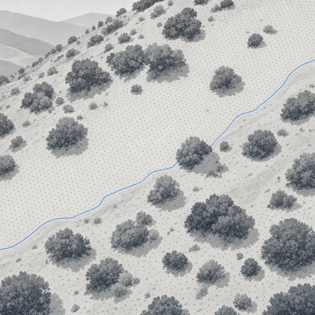
A scope of work says "minimum 100 points per square meter." Another says "QL1." A third says nothing about density at all. All three leave the same question open: will the surface you design from be good enough where it matters?
This post separates three numbers that get mixed up (pulses, points and ground points), shows what they look like in real public lidar from Los Angeles, Palm Beach County and the Atlanta area, and ends with scope language that asks for the deliverable instead of a density.
Three numbers that share one unit
"Points per square meter" can mean three different things.
- Pulse density. First returns per square meter. One pulse, one first return. This is what the USGS and ASPRS standards count.
- Total point density. Every return per square meter. A pulse that hits a branch and then the ground yields two points. A sensor with multiple returns, such as the DJI Zenmuse L2, lists a maximum of 240,000 points per second on a single return and 1,200,000 on multiple returns, so a "total" figure can be several times the pulse figure.
- Ground point density. Points classified as bare earth. This is the number that builds a DTM, contours and cut/fill volumes.
The three agree on open pavement and diverge fast under vegetation. A spec that names one without the others is easy to satisfy on paper and still deliver a thin surface where the site is hard.
What USGS 3DEP actually requires
The USGS Lidar Base Specification sets density by quality level. Its table 1, in version 1.3 (February 2018), reads as follows. Table 4 of the same document gives the accuracy that goes with each level.
| Quality level | Min. aggregate nominal pulse density | Max. pulse spacing | RMSEz (nonvegetated) | VVA, 95th percentile |
|---|---|---|---|---|
| QL0 | 8 pulses/m² | 0.35 m | 5 cm | 15 cm |
| QL1 | 8 pulses/m² | 0.35 m | 10 cm | 30 cm |
| QL2 | 2 pulses/m² | 0.71 m | 10 cm | 30 cm |
| QL3 | 0.5 pulses/m² | 1.41 m | 20 cm | 60 cm |
Two details are worth reading twice.
First, QL0 and QL1 have the same density. QL0 differs by accuracy, a 5 cm RMSEz instead of 10 cm. A common misreading treats QL0 as "denser than QL1." It is not, in this version of the specification. The specification itself says the QL0 requirements are "somewhat arbitrary" and may change. A newer revision may differ, so check the current edition before you quote a table in a contract.
Second, the unit is pulses, counted from first returns. The specification also says that, "dependent on the local terrain and land cover conditions in a project, a greater pulse density may be required." In other words, the number is a floor for the whole project, not a promise about ground points under a stand of oak.
What real 3DEP data looks like
To see how the three numbers behave, this post reads a 300 m by 300 m window of public 3DEP point cloud at four sites from the USGS lidar bucket on AWS and counts points in each class.

The numbers, from the Los Angeles, Palm Beach and Georgia project files:
| Window | First returns/m² | All returns/m² | Ground points/m² | 1 m cells with no ground point |
|---|---|---|---|---|
| Palm Beach County, flat farmland (2019 project) | 17.2 | 23.0 | 11.2 | 7% |
| Los Angeles, open parkland (B23 project) | 14.6 | 15.8 | 11.1 | 3% |
| Los Angeles, chaparral hillside (B23 project) | 20.0 | 26.1 | 7.4 | 18% |
| Atlanta area, forest (2018 statewide project) | 2.1 | 4.3 | 0.49 | 68% |
Three things stand out.
- The chaparral window beats QL1 on pulses and still has 18% of its 1 m cells empty of ground points. It has 20 first returns per square meter, but only 28% of its points are ground. The window also takes in the Griffith Observatory building and grounds. Setting aside a 70 m box around the building still leaves about 15% of 1 m cells empty, a rough check. A spec of "8 pulses/m²" is met by a wide margin and says little about the surface.
- The forest window meets QL2 on pulses (2.1 against a minimum of 2) and has 0.49 ground points per square meter. That is the kind of coverage a QL2 collection gives under a closed canopy. It is a single window, not a statement about all of Georgia.
- ASPRS has a name for this. Its Edition 2 standard suggests flagging low confidence areas where ground density falls to a quarter or less of the recommended pulse density. For a 10 cm class (2 pulses/m²), that threshold is 0.5 ground points per square meter. The Atlanta window sits right at it.
The collection dates are inferred from the GPS time stamps in the files (see the notes at the end), and these are airborne collections, not drone data. They are useful here because they are public, and because the same mechanics apply to any lidar.
Where the ground points are
An average hides the pattern. Figure 2 maps ground points per 2 m cell for two of the windows.

The open window is dense almost everywhere, with a few bare patches. The chaparral window ranges from nothing to more than 20 points per square meter within a few tens of meters. Dense bands in both maps appear to follow where flight lines overlap, an inference from the pattern that was not checked against flight-line metadata. The empty patches in the chaparral map have causes that cannot be separated from the point cloud alone: roofs, water and dense cover all leave no ground points. The large empty block near the center is the observatory building.
What density buys
Does more density buy a better surface? It depends on the ground. A simple test on the same data gives a sense of it. For each site, 10% of the ground points in a central 150 m by 150 m box were held out as checkpoints. The rest were thinned at random to a lower density, triangulated into a surface, and compared with the checkpoints. Because of the smaller box and the hold-out, the starting densities differ from the table above.

| Site | Full ground density (points/m²) | Error at full density | Density after thinning | Error after thinning |
|---|---|---|---|---|
| Palm Beach farmland | 13.4 | 1.8 cm | 1.7 | 2.1 cm |
| LA open parkland | 11.5 | 2.0 cm | 1.4 | 4.0 cm |
| LA chaparral | 7.0 | 3.0 cm | 1.8 | 5.5 cm |
| Atlanta forest | 0.43 | 4.8 cm | 0.11 | 11.6 cm |
On flat farmland, cutting the density by a factor of eight added about 0.3 cm. On the chaparral hillside, cutting it by a factor of four nearly doubled the error. In the forest the error was already 4.8 cm at full density and about 12 cm after thinning.
This test has limits. The reference is the same dataset, so it measures what thinning loses, not absolute accuracy. Random thinning is kinder than a real, clumpy return pattern. And the checkpoints are points the sensor did find on the ground, so the forest figures are optimistic about places where it found none.
The pattern is the point. Density matters most where the ground is rough or covered. That is where a flat "points per square meter" number is least informative.
Drone lidar sits in a different regime
Drone sensors fly low and slow, so their numbers look different. A Caltech team surveying post-fire debris basins in Los Angeles County flew a DJI Zenmuse L2 at 100 to 120 m above ground, with 80% front overlap and 20% lateral overlap. That configuration gave 500 to 700 points per square meter and an elevation error of 2 to 3 cm over bare ground (Chen et al., Landslides, 2026).
Compare that with an independent test of the same sensor. Tamimi and Toth, in the ISPRS Archives (2024), built a DTM from a ground-classified cloud of about 725 points per square meter. They checked it against total-station points. The error was about 7 cm on an open road and about 21 cm under forest canopy.
Density in the hundreds per square meter did not remove the canopy error. DJI's own system figure for the L2 is 4 cm vertical and 5 cm horizontal at 150 m, measured in a laboratory. ASPRS makes the same point in its Edition 2 appendix: increasing point density "does not change the system error." What denser data does is make the surface between points more faithful, especially for curbs and small drainage features, and, under vegetation, make it more likely that some pulses reach the ground.
A surveyor made a related point about accuracy in a vendor-hosted video. Daniel Cooper, a Texas surveyor with 23 years in the field, put it this way: "i don't know that the drone is going to be more accurate than traditional surveying methods but it's going to eliminate some of the systematic errors."
What the standards recommend
ASPRS Edition 2 gives a recommended minimum pulse density for each vertical accuracy class in its table B.9. It adds that users "may select higher or lower point densities to best fit project requirements and complexity of surfaces to be modeled."
| Vertical accuracy class (NVA) | Recommended min. pulse density | Max. pulse spacing |
|---|---|---|
| 2.5 cm | 16 pulses/m² | 0.25 m |
| 5 cm | 8 pulses/m² | 0.35 m |
| 10 cm | 2 pulses/m² | 0.71 m |
| 20 cm | 0.5 pulses/m² | 1.4 m |
Density and spacing are linked by spacing = 1 / square root of density, which is the same relation both standards use. By that arithmetic, 25 points per square meter is a 20 cm average spacing, 100 is 10 cm and 500 is about 4.5 cm. That is average spacing, not the spacing along a curb line. A 15 cm curb face is a poor match for 20 cm spacing, which is why features are better specified as features than as a density.
The storage cost is real, but it is the smaller problem
Density has a file cost. The table below is arithmetic: points on 50 acres, times bytes per point for LAS 1.4 point formats 6 and 7, which are among the formats the USGS specification allows. It assumes uncompressed files and ignores LAZ compression.
| Density | Points on 50 acres | LAS 1.4 format 6 (30 bytes/point) | Format 7, with RGB (36 bytes/point) |
|---|---|---|---|
| 8 points/m² | 1.6 million | 0.05 GB | 0.06 GB |
| 100 points/m² | 20 million | 0.61 GB | 0.73 GB |
| 500 points/m² | 101 million | 3.0 GB | 3.6 GB |
A 3 GB cloud is manageable for a data team and unpleasant for a designer's laptop. The bigger cost is downstream: a classified, thinned surface is what most design software wants. One option is to deliver the full-density classified cloud as the record and a thinned ground layer for design. Ask for both if you want to keep the option.
What to write in the scope instead
A provider who used to be the buyer has said it plainly. Daniel Windham, who runs a drone-LiDAR firm in Georgia and has said he used to hire people to do this work, said: "nobody cares what drone you're running unless it's in their SOP." Buyers care about the deliverable.
A scope that names the deliverable gives the provider room to choose the sensor, altitude and overlap, and gives you something you can check. Consider asking for:
- An accuracy class and how it will be tested. For example, a stated vertical class with RMSEv reported separately for open ground and vegetated areas. ASPRS Edition 2 calls for at least 30 checkpoints for a fully compliant assessment and treats vegetated vertical accuracy as a value to report, not a pass/fail test.
- Ground point density, reported. Ask for the average and a raster of ground points per square meter, with a cell size you name. Spot cells below your threshold, such as 25% of the target pulse density, as low-confidence areas.
- Feature requirements. Breaklines for curbs, walls, channel banks and pavement edges, with a vertex spacing, rather than a density meant to capture them by accident.
- Surface and file deliverables. Classified point cloud (ground, vegetation, noise), a DTM at a stated cell size and the coordinate system and vertical datum, plus the thinned ground layer your software prefers.
- A land-cover note. If the site has brush or trees, say so, and say how much of the design rests on ground under it. If it matters, plan conventional shots under cover as an add to the lidar, not instead of it.
Sample language: "The DTM shall meet a stated vertical accuracy class tested against no fewer than 30 independent checkpoints, with vegetated areas reported separately. The provider shall deliver a raster of ground-point density and shall identify areas below the stated minimum. Breaklines shall be delivered at curbs, walls and channel banks."
Compare that with "minimum 400 points per square meter." It might be necessary on a facade. It might be ten times more than a grading surface on open ground needs, and it says nothing about the hillside cells with no ground point.
A note on who signs
A topographic surface delivered for design or a permit needs a licensee in responsible charge. In California that is a PLS, or a civil engineer legally authorized to practice land surveying. In Georgia it is a PLS. In Florida it is a PSM. Twinn Digital does not stamp. It captures and processes the data, and a licensed partner reviews and signs. If the work is federally funded, check SAM.gov for current restrictions on the aircraft and sensor before you name one in a scope. The compliance page lists what Twinn can and cannot do.
Next step
Pick one open project you are about to scope. Replace the density line with an accuracy class, a ground-density report and a short feature list, then send it to your provider and see what comes back. Twinn Digital rents equipment per job and does not tie a scope to one sensor, so a scope written to the deliverable fits its workflow. If you are a surveyor or civil firm with a scope to check, the surveyors and engineers page is a place to start.
How the data in this post was handled
The density windows, maps and thinning test were built from the public 3DEP files with a short script, and can be rebuilt from them. Collection dates come from the files' GPS time stamps, assuming the usual adjusted standard GPS time. Treat them as approximate. The 3DEP windows are airborne lidar and stand in for the general behavior of lidar, not for any drone survey.